When Better BSR Makes You Less Money: A Quantitative Framework for Amazon PPC Profitability

In contemporary e-commerce architecture and advertising diagnostics, a persistent operational fallacy continues to drain enterprise capital: the unconstrained pursuit of Best Sellers Rank (BSR) under the naive assumption that top-line scale intrinsically guarantees bottom-line expansion. Operational teams routinely deploy aggressive advertising budgets to force BSR progression without evaluating whether the marginal sales volume covers the incremental advertising friction.

This paper establishes a closed mathematical diagnostic framework connecting search ranking dynamics directly to unit economics and net profit optimization. By establishing deterministic algebraic bridges between BSR, daily unit shipment volume ($V$), baseline gross margin ($M_{\text{gross}}$), and Total Advertising Cost of Sales ($\text{TACoS}$), we derive a universal mathematical boundary ($\Delta\text{TACoS}_{\max}$) that dictates precisely when advertising expenditure turns value-destructive.

1. Equation 1: BSR-to-Volume Power-Law Conversion Model

Marketplace sales velocity across categories does not scale linearly; volume distribution across ranking positions follows a continuous heavy-tailed power-law function. The non-linear decay of daily shipment volume relative to numeric BSR position ($R$) is formulated as:

$$V = \alpha \cdot R^{-\gamma}$$

Variable Definitions & Operational Parameters

• $V$: Estimated daily shipment volume ($\text{units/day}$).
• $R$: Best Sellers Rank numerical index ($R \in \mathbb{Z}^+$, where $R=1$ represents the category leader).
• $\alpha$ (Category Ceiling Coefficient): Theoretical daily volume output of the rank 1 listing ($R=1$) within a specific sub-category niche.
• $\gamma$ (Power-Law Decay Exponent): Empirical slope coefficient reflecting market consolidation and top-heavy volume concentration.

Structural First-Principles of Power-Law Decay

To firmly ground the mathematical framework, we establish the structural mechanics governing why category volume distribution strictly adheres to power-law decay across three continuous system dynamics:

1. Attention & Click Concentration Dynamics (SERP Architecture)

Amazon’s Search Engine Results Page (SERP) is inherently top-heavy. Consumer eye-tracking and placement conversion data reveal that user engagement drops precipitously below top organic positions. Page 1 top-of-search slots capture the overwhelming majority of buyer intent. Because search engine layouts funnel impressions into discrete top placements, traffic distribution inherently assumes a heavy-tailed profile.

2. Network Effects & Preferential Attachment

The Amazon ranking algorithm relies on a compounding positive feedback loop: higher sales velocity generates stronger conversion signals, prompting the system to assign greater organic real estate and placement priority. In complex algorithmic ecosystems, this preferential attachment mechanism (“the rich get richer”) mathematically dictates a power-law distribution.

3. Empirical Pareto Distribution Across Niche Micro-Ecosystems

Across standard Amazon sub-categories, market share mirrors the generalized Pareto principle: the top 20% of listings systematically secure ~80% of total category volume. The power-law formulation provides a practical way to approximate this highly skewed volume distribution this extreme volume skew seamlessly across both top-tier (#1–#10) and long-tail (#100+) positions.

Operational Parameter Calibration via Log-Log OLS Regression

In Equation 1, the model depends on two deterministic parameters: the Category Ceiling Coefficient ($\alpha$) and the Power-Law Decay Exponent ($\gamma$). Rigorous quantitative modeling avoids arbitrary static assumptions, deriving both parameters directly from empirical marketplace data for each specific ASIN and sub-category.

By taking the natural logarithm ($\ln$) of both sides of Equation 1, we transform the non-linear power curve into a simple linear equation:

$$\ln(V) = \ln(\alpha) – \gamma \cdot \ln(R)$$

This maps directly to standard simple linear regression:

$$Y = a + bX$$

Where:

• $Y = \ln(V)$
• $X = \ln(R)$
• $a = \ln(\alpha) \quad \implies \quad \alpha = e^a$
• $b = -\gamma \quad \implies \quad \gamma = -b$

Empirical Calibration Protocol for Operators:

1. Extract Historical Pairs: Gather 30 or 60 days of daily BSR ($R$) and daily unit volume ($V$) for your listing (excluding abnormal promo spikes or stockouts).
2. Transform Data: Compute $\ln(R_t)$ and $\ln(V_t)$ for each data point $t$.
3. Run OLS Regression: Execute an Ordinary Least Squares (OLS) regression on the transformed dataset in Excel or Python.
4. Verify Goodness-of-Fit ($R^2$): A coefficient of determination $R^2$ > 0.85 can be used as a practical threshold for evaluating the fit of this power-law framework.
5. Extract Parameters: Read slope $b$ to establish exact category decay $\gamma = -b$, and compute $\alpha = e^a$.

Step-by-Step Numerical Walkthrough

Consider a niche category calibrated via historical regression where $\alpha = 500$ (the #1 best seller outputs 500 units/day) and $\gamma = 0.60$.

State A: Baseline Rank Position ($R_1 = 20$)

$$V_1 = 500 \cdot (20)^{-0.60} = 500 \cdot (0.164938) \approx 82.5 \text{ units/day}$$

State B: Accelerated Rank Position ($R_2 = 10$)

$$V_2 = 500 \cdot (10)^{-0.60} = 500 \cdot (0.251188) \approx 125.5 \text{ units/day}$$

Diagnostic Conclusion 1: Advancing BSR position from 20 to 10 delivers an incremental throughput of:

$$\Delta V = 125.5 – 82.5 = 43.0 \text{ units/day } (+52.12\% \text{ volume growth})$$

Equation 1 converts an abstract rank numeric into an exact physical throughput metric ($V$).

2. Equation 2: Daily Net Profit Expansion & Unit Economics

Converting daily unit volume ($V$) into net operational returns requires accounting for unit price, gross margins, and advertising drag. Net profit per day ($\Pi_{\text{net}}$) is defined as:

$$\Pi_{\text{net}} = V \cdot P \cdot (M_{\text{gross}} – \text{TACoS})$$

Variable Definitions

• $\Pi_{\text{net}}$: Net daily operational profit ($\text{USD/day}$).
• $P$: Selling price per unit ($\text{USD}$). Assumed constant at $\$30.00$.
• $M_{\text{gross}}$: Baseline Gross Margin percentage prior to advertising spend, defined as:

$$M_{\text{gross}} = \frac{P – \text{COGS} – \text{FBA Fees} – \text{Referral Fees} – \text{Freight}}{P}$$

Assumed fixed at $30.00\%$ ($0.30$).

• $\text{TACoS}$: Total Advertising Cost of Sales ratio, defined as:

$$\text{TACoS} = \frac{\text{Total Advertising Spend}}{\text{Total Gross Revenue}}$$

Comparative Scenario Analysis: The BSR Ranking Trap

To demonstrate how aggressive rank expansion can erode bottom-line profit when advertising spend scales without algebraic constraints, we evaluate the two operational states derived from Equation 1:

Metric Parameter	Scenario A (Restrained Ad Strategy)	Scenario B (Aggressive Rank Push)
BSR Position ($R$)	$R_1 = 20$	$R_2 = 10$
Daily Volume ($V$)	$82.5 \text{ units/day}$	$125.5 \text{ units/day}$
Selling Price ($P$)	$\$30.00$	$\$30.00$
Daily Gross Revenue ($V \cdot P$)	$\$2,475.00$	$\$3,765.00$
Baseline Gross Margin ($M_{\text{gross}}$)	$30.00\% \ (0.30)$	$30.00\% \ (0.30)$
Realized TACoS	$10.00\% \ (0.10)$	$25.00\% \ (0.25)$
Net Operational Margin ($M_{\text{gross}} – \text{TACoS}$)	$20.00\% \ (0.20)$	$5.00\% \ (0.05)$
Daily Net Profit ($\Pi_{\text{net}}$)	$\$495.00 / \text{day}$	$\$188.25 / \text{day}$

Diagnostic Takeaway: Despite driving an additional $\$1,290.00$ in daily top-line revenue ($+52.12\%$) and climbing 10 places up the category rank, daily net cash flow collapsed by $-\$306.75 / \text{day}$ (a $-61.97\%$ destruction in net daily profit). Top-line growth masked severe bottom-line margin erosion.

3. Equation 3: Mathematical Derivation of the TACoS Upper Bound

To eliminate trial-and-error ad expenditure, operators must isolate the exact mathematical boundary where a rank push yields non-negative incremental net profit ($\Delta\Pi_{\text{net}} > 0$).

First-Principles Algebraic Derivation

Let baseline parameters be defined by $V_1, \text{TACoS}_1, \Pi_{\text{net},1}$.

Let target state parameters be defined by $V_2, \text{TACoS}_2, \Pi_{\text{net},2}$.

For rank advancement to expand net profit, the profit delta must strictly exceed zero:

$$\Delta\Pi_{\text{net}} = \Pi_{\text{net},2} – \Pi_{\text{net},1} > 0$$

Substitute Equation 2 into the inequality:

$$V_2 \cdot P \cdot (M_{\text{gross}} – \text{TACoS}_2) – V_1 \cdot P \cdot (M_{\text{gross}} – \text{TACoS}_1) > 0$$

Since $P > 0$, divide both sides by $P$:

$$V_2 \cdot (M_{\text{gross}} – \text{TACoS}_2) – V_1 \cdot (M_{\text{gross}} – \text{TACoS}_1) > 0$$

Define target $\text{TACoS}_2$ as baseline $\text{TACoS}_1$ plus an allowable expansion buffer $\Delta\text{TACoS}$:

$$\text{TACoS}_2 = \text{TACoS}_1 + \Delta\text{TACoS}$$

Substitute this into the inequality:

$$V_2 \cdot \left(M_{\text{gross}} – (\text{TACoS}_1 + \Delta\text{TACoS})\right) – V_1 \cdot (M_{\text{gross}} – \text{TACoS}_1) > 0$$

Expand and rearrange terms:

$$V_2 \cdot (M_{\text{gross}} – \text{TACoS}_1) – V_2 \cdot \Delta\text{TACoS} – V_1 \cdot (M_{\text{gross}} – \text{TACoS}_1) > 0$$

Group like terms:

$$(V_2 – V_1) \cdot (M_{\text{gross}} – \text{TACoS}_1) > V_2 \cdot \Delta\text{TACoS}$$

Divide both sides by $V_2$ (since $V_2 > 0$):

$$\Delta\text{TACoS} < (M_{\text{gross}} – \text{TACoS}_1) \cdot \left(1 – \frac{V_1}{V_2}\right)$$

Step-by-Step Numerical Calibration

Plugging in our operational baseline parameters ($V_1 = 82.5$, $V_2 = 125.5$, $M_{\text{gross}} = 0.30$, $\text{TACoS}_1 = 0.10$):

1. Volume Retention Ratio:
   $$\frac{V_1}{V_2} = \frac{82.5}{125.5} \approx 0.65737$$
2. Volume Growth Retention Factor:
   $$1 – \frac{V_1}{V_2} = 1 – 0.65737 = 0.34263$$
3. Baseline Net Margin Buffer:
   $$M_{\text{gross}} – \text{TACoS}_1 = 0.30 – 0.10 = 0.20 \ (20.00\%)$$
4. Maximum Allowable TACoS Expansion ($\Delta\text{TACoS}_{\max}$):
   $$\Delta\text{TACoS}_{\max} = 0.20 \cdot 0.34263 = 0.06852 \quad (6.85\%)$$
5. Absolute Upper Bound Target TACoS ($\text{TACoS}_{2,\max}$):
   $$\text{TACoS}_{2,\max} = \text{TACoS}_1 + \Delta\text{TACoS}_{\max} = 10.00\% + 6.85\% = \mathbf{16.85\%}$$

Diagnostic Conclusion 2: To ensure that pushing BSR from position 20 to 10 generates positive incremental net cash flow, total account TACoS cannot exceed 16.85%. In Scenario B, when TACoS rose to 25.00%, it breached this ceiling by 8.15 percentage points, destroying profitability.

4. Operational Synthesis & Execution Protocol

This framework unifies market position, advertising expense, and net cash flow into a deterministic operational execution loop:

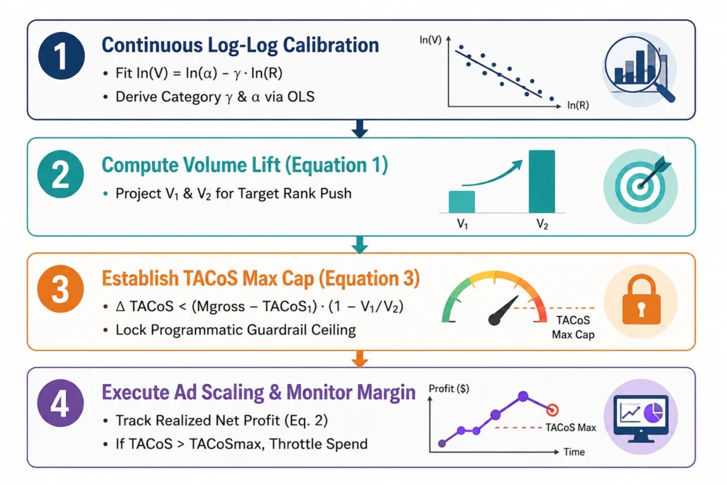
1. Continuous Data Calibration: Perform OLS regression on historical $\ln(V)$ vs. $\ln(R)$ pairs to confirm local $\gamma$ and $\alpha$ coefficients before altering campaign bidding structures.
2. Volume Throughput Projection: Input target BSR ranking ($R$) into Equation 1 to establish baseline unit throughput expectations.
3. Upper-Bound Risk Control: Compute $\Delta\text{TACoS}_{\max}$ and set programmatic account-level ad spend guardrails at $\text{TACoS}_{2,\max}$ prior to launching ranking pushes.
4. Real-Time Profit Validation: Monitor realized performance via Equation 2. If campaign scaling fails to keep total TACoS below $\text{TACoS}_{2,\max}$, immediately reduce ad spend to baseline levels to prevent capital erosion.

Disclaimer & Model Operational Boundaries

1. Analytical Tool, Not a Guarantee of Profitability

The quantitative framework, linear regressions, and TACoS ceiling equations presented in this document offer a structured, mathematically rigorous methodology for diagnosing Amazon PPC efficiency and rank economics. However, this framework represents an abstraction of complex marketplace behavior. It does not guarantee specific financial outcomes or automatic profitability.

2. Exogenous Noise Variables & Market Volatility

Real-world e-commerce performance is continuously influenced by uncontrolled, high-entropy noise variables. These include—but are not limited to—category seasonality, dynamic competitor pricing strategies, Buy Box suppression, inventory stockouts, sudden conversion rate shifts, and updates to Amazon’s underlying search and recommendation algorithms. No mathematical equation can fully isolate or predict all exogenous shocks.

3. Necessity of Dynamic Calibration

The eco-coefficients ($\alpha$ and $\gamma$) defined within this model are strictly time-bound and context-dependent. They are not static constants. Users must treat this model as a living operational system, requiring routine monthly re-regression against updated 30-day trailing datasets to ensure predictive alignment with evolving market conditions.

This framework serves as an advanced decision-support instrument to establish disciplined risk boundaries—it is designed to augment, not replace, experienced operational judgment.

5. Frequently Asked Questions (FAQ) & Continuous Calibration Protocol

Q1: Are the $\alpha$ and $\gamma$ coefficients fixed values that only need to be computed once?

A: Absolutely not. $\alpha$ and $\gamma$ are dynamic eco-coefficients that must be recalibrated regularly on a 30-day (monthly) cycle.

• Why static values fail: As your listing climbs in rank, accumulates account authority, shifts advertising strategies, or as category competitors adjust their operations, the underlying dataset evolves. Parameters computed during an earlier launch phase will inevitably lose predictive precision two to three months later.
• Recalibration Direction: Operators should establish a 30-day evaluation cadence, pulling real daily shipment and BSR scatter data from the trailing month to re-run OLS regressions and update $\alpha$ and $\gamma$.
• Core Philosophy: This diagnostic framework is not a static formula, but an active, living operational system. Systematic monthly recalibration guarantees that your derived TACoS ceilings remain tightly aligned with live category dynamics rather than outdated assumptions.

Q2: What software tools can be integrated with this model for efficient execution?

A: We recommend integrating Nova Data—specifically leveraging its BSR Tracker module—to streamline operational workflow.

• System Integration Logic: The primary input requirements for this diagnostic model are continuous, high-fidelity BSR rank trajectories and sales volume trends.
• How Nova Data Supports the Framework:
  1. Granular BSR Monitoring: Nova Data’s BSR Tracker automatically captures and cleans historical BSR fluctuation curves for your ASIN and key category competitors, removing the manual overhead of daily rank tracking.
  2. High-Quality Regression Inputs: Its historical tracking archives deliver clean, unpolluted data pairs required for monthly OLS regression runs. This allows operators to bypass manual data collection and focus strictly on executing parameter recalibrations and enforcing TACoS risk ceilings.